HNSW Vector Search Explained: The Shortcut Graph Behind Fast Retrieval

20 Sep

HNSW vector search is one of the quiet constraints behind a useful RAG system. A support assistant with a few hundred document chunks can compare a question with every chunk. At millions of vectors, that simple approach turns every question into a large numerical scan.

Hierarchical Navigable Small World graphs, usually shortened to HNSW, offer a different route. They build a navigable graph over embeddings so a query can move quickly towards a promising part of vector space, then search the local neighbourhood in more detail. The result is fast approximate nearest-neighbour search, not a guarantee of the mathematically exact answer.

This article explains what the hierarchy does, how insertion and search work, which parameters matter, and where HNSW needs careful system design in a production RAG application.

Why exact vector search does too much work

Embedding models map text, images, or other inputs to numerical vectors. When a question and a document chunk have related meaning, their vectors should be close under a chosen distance or similarity metric. A vector database can therefore retrieve candidate evidence before an LLM writes an answer.

The exact method is straightforward: calculate the query’s distance to every stored vector and take the nearest k. It is a valuable evaluation baseline, but its cost grows with the collection. HNSW searches only a subset of nodes in an index graph. Microsoft’s vector-search documentation describes this contrast directly: exhaustive k-nearest-neighbour search evaluates all neighbours, while HNSW searches a graph over a subset of nodes.

Compression is another lever when storage is the problem. It is related, but not the same as HNSW. For that distinction, see Vector Quantisation: How Code Books Compress Similar Data.

HNSW vector search in one picture: motorways above local streets

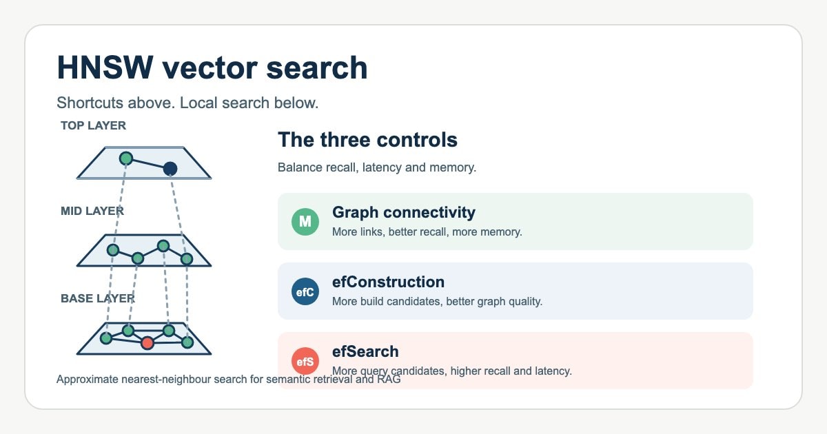
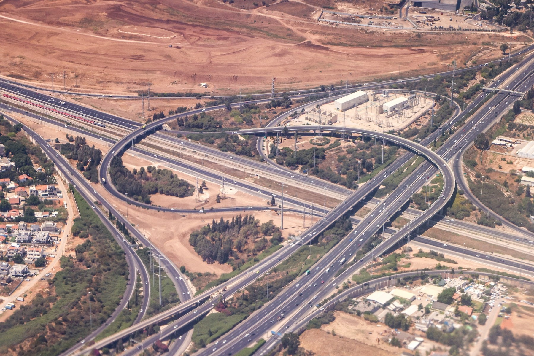
A useful analogy is a road network. You would not drive every street in a country to reach a restaurant. You use motorways to cross distance quickly, take regional roads to reach the right area, then use local streets for the final approach.

HNSW applies this idea to a hierarchy of proximity graphs:

• Layer 0 contains every indexed vector and supports detailed local search.
• Higher layers contain progressively smaller, nested subsets of those vectors.
• Edges connect selected nearby vectors according to the configured metric, such as cosine distance or Euclidean distance.

The original HNSW paper specifies that a vector’s highest layer is selected randomly with an exponentially decreasing probability. That is why upper layers have fewer nodes. The hierarchy separates links by characteristic distance scale, making it possible to make broad progress before local refinement.

How HNSW vector search finds neighbours

Consider a hypothetical internal-support assistant with ten million authorised document chunks. A user asks, “How do I reset a customer password when MFA is unavailable?” The application embeds the question and sends the vector to the index.

1. Enter at the highest layer. The search starts from the index entry point in the top available layer.
2. Move greedily while the layer is coarse. It follows a neighbouring node if that node is closer to the query under the selected metric. When no neighbour improves the result, it stops at that layer.
3. Descend one layer. The best position found becomes the entry point for the next, denser layer.
4. Explore candidates at the base layer. Instead of returning one node after a simple walk, the search maintains a bounded candidate set. It expands promising candidates and retains the best results found.
5. Return the top k. The application receives document IDs and distances, then can apply retrieval policy, reranking and answer generation.

This last step matters. HNSW is a retrieval component, not permission enforcement. The tenant, user, document status and other access boundaries must be designed so an unauthorised chunk cannot become evidence for an answer.

Why “approximate” is an engineering choice

HNSW does not promise the exact nearest neighbours for every query. It makes a deliberate recall, latency and memory trade-off. A query may miss a relevant chunk if the graph is under-built, the search breadth is too small, the embedding space is difficult to navigate, or filters remove candidates after retrieval.

That does not make HNSW unreliable. It means quality has to be measured. Build an evaluation set from representative questions, establish an exact-search ground truth, and report Recall@k alongside latency. A useful production target is not “the index is fast”; it is “the evidence needed by this application appears in the retrieval set often enough, within the latency budget.”

HNSW vector search parameters that change the trade-off

The hnswlib implementation documents the same split. It describes ef as the dynamic list size during search, M as the number of bidirectional links created during construction, and ef_construction as the construction-time speed and accuracy control.

Do not copy a parameter tuple from a benchmark and call it tuned. Dataset size, dimensionality, the query distribution, the chosen metric, available memory and the required recall all change the answer. Start with sensible library defaults, measure exact recall on your own data, then adjust one factor at a time.

A small hnswlib example

import hnswlib

# Example only. Use the dimension and metric that match the embedding model.
index = hnswlib.Index(space="cosine", dim=1536)

index.init_index(
    max_elements=1_000_000,
    M=16,
    ef_construction=200,
)

index.add_items(document_embeddings, document_ids)

# Query-time recall and latency control. Keep ef at least as large as k.
index.set_ef(100)
labels, distances = index.knn_query(question_embedding, k=5)

The code is intentionally short because the configuration needs an experiment, not a universal prescription. Record the embedding model, metric, index settings, hardware, dataset version and evaluation queries alongside any recall result.

HNSW insertion: online, but not free

HNSW supports incremental insertion. For each new vector, the index samples a maximum level, traverses the existing graph to find candidate neighbours, selects links using a proximity heuristic, and updates the relevant layers.

This is useful for a knowledge base that receives new documents throughout the day. It does not mean the index automatically maintains identical performance under every workload. Large ingestions, data that arrives in a skewed order, changed embedding models, deletions and changing query patterns all deserve testing. In many systems, rebuilding an index after a major corpus or embedding change is a sensible operational option.

HNSW vector search in a RAG pipeline

Return to the password-reset question. A robust pipeline could look like this:

1. Chunk and embed authorised support content.
2. Use HNSW to retrieve a wider candidate set, for example 20 chunks.
3. Apply access control and product or tenant constraints.
4. Combine vector and keyword results when exact product names, error codes or policy numbers matter.
5. Rerank the remaining candidates with a stronger relevance model or an application-specific rule.
6. Pass only the best, permitted evidence to the LLM, with citations where the product supports them.
7. Evaluate whether the required source appeared in the set, not merely whether the final answer sounded plausible.

HNSW can make step two fast. It cannot repair weak chunking, an unsuitable embedding model, stale documents, a missing filter, or a hallucinated final answer. Microsoft’s guidance similarly recommends testing chunk size and overlap, increasing k where appropriate, and considering hybrid queries and semantic ranking when relevance is poor.

HNSW vector search and the filtered-results trap

Filtering is where a neat nearest-neighbour demo becomes a real system-design problem. Imagine that the application shares one index across customers and asks for five results only from tenant_id = 42.

SELECT id, content
FROM knowledge_chunks
WHERE tenant_id = 42
ORDER BY embedding <=> :query_embedding
LIMIT 5;

In approximate search, an engine may scan vector candidates and apply the filter afterwards. If only ten percent of candidates belong to the tenant and the candidate budget is small, the query can return fewer permitted results than expected. The pgvector documentation gives this exact example: with a ten-percent filter and its default HNSW search breadth of 40, only about four rows match on average.

Possible responses include increasing query breadth, enabling iterative scans where the database supports them, indexing the filter column, using partial indexes for a small set of values, or partitioning data. The right choice depends on selectivity, workload and the required isolation boundary. Never solve the symptom by weakening tenant access control.

When HNSW is a good fit, and when it is not

HNSW is often a strong option for low-latency semantic search with a substantial vector collection, high recall expectations and frequent queries. It is especially attractive when new vectors must be inserted without training a separate coarse quantiser first.

It may be a weaker fit when exact answers are mandatory, RAM is tightly constrained, filtering dominates every query, or index construction cost is the primary concern. Other options include exhaustive search for small collections, inverted-file indexes, quantised indexes and disk-oriented vector-search designs. The choice should follow measurements, not a fashionable default.

Closing thought

HNSW earns its place because it changes vector search from “compare with everything” to “navigate toward the right neighbourhood.” The upper layers supply shortcuts, while the base layer supplies the detail.

For an engineer building RAG, the practical lesson is wider: tune graph construction and search against an exact baseline, build access boundaries into the retrieval path, and evaluate the evidence retrieved before celebrating the answer generated.

Further reading

• Malkov and Yashunin, Efficient and Robust Approximate Nearest Neighbor Search Using Hierarchical Navigable Small World Graphs
• hnswlib algorithm parameters
• pgvector HNSW, filtering and iterative scan documentation
• Microsoft Learn: Vector relevance and ranking